What the Binomial Model Does
The binomial option pricing model, developed by Cox, Ross, and Rubinstein in 1979, breaks the time until an option’s expiration into a series of discrete steps. At each step, the underlying asset’s price is assumed to move either up or down by a specific factor, building out a branching ‘tree’ of possible price paths. The option’s value at each final node is calculated first, then worked backward through the tree, discounting at each step, to arrive at today’s fair value.
What Black-Scholes Does Differently
The Black-Scholes model, published in 1973, instead assumes the underlying price moves continuously and follows a specific statistical distribution (geometric Brownian motion), which allows the option’s fair value to be computed with a single closed-form equation — no step-by-step tree required. It’s faster to compute but, in its basic form, values only European-style options that can be exercised solely at expiration.

Why Binomial Trees Handle American Options Better
Because the binomial model evaluates the option’s value at every intermediate node in the tree, it can directly compare ‘exercise now’ versus ‘hold and continue’ at each step and pick whichever is more valuable. That makes it naturally suited to American-style options, which can be exercised any time before expiration. Black-Scholes’ single-formula approach has no mechanism to check for early exercise, so it isn’t built for that job without modification.
The Two Models Converge as Steps Increase
As the number of steps in a binomial tree increases toward infinity, its calculated option value converges to the Black-Scholes price for a European option. In that sense, the binomial model can be thought of as a discrete-time approximation of Black-Scholes — the two aren’t competing theories so much as complementary tools suited to different practical needs.
| Feature | Binomial Model | Black-Scholes Model |
|---|---|---|
| Price movement assumption | Discrete (up/down steps) | Continuous (geometric Brownian motion) |
| Calculation method | Step-by-step tree, worked backward | Single closed-form formula |
| American-style options (early exercise) | Handles directly | Not handled without modification |
| Computation speed | Slower with more steps | Very fast |
Frequently Asked Questions
How many steps does a binomial tree typically need?
In practice, 50 to 100 steps or more are commonly used to get results that closely approximate the Black-Scholes value for a comparable European option. Too few steps can leave meaningful pricing error.
How are the up and down factors chosen in a binomial tree?
The Cox-Ross-Rubinstein approach commonly sets the up factor as u = e^(σ√Δt) and the down factor as d = 1/u, where σ is the underlying’s volatility and Δt is the length of each step — larger volatility produces wider up and down swings.
Is the binomial model used for anything besides options?
Yes. The same tree-based logic is used to value convertible bonds, warrants, and real options in corporate finance, such as the option value embedded in a phased capital investment decision.
Which model do professional trading desks actually use?
Many desks use both, along with more advanced numerical methods, depending on the instrument: Black-Scholes-type closed forms for quick European option pricing, and binomial or other tree/lattice methods when early exercise or other path-dependent features need to be captured.
Key Takeaways
The binomial model breaks an option’s life into discrete steps and builds a price tree that can directly account for early exercise, making it well suited to American-style options. Black-Scholes instead solves for a European option’s value in one closed-form calculation, and as the binomial tree’s step count grows, its result converges toward the Black-Scholes price — making the two models complementary rather than opposing approaches. This article is for informational purposes only and does not constitute investment advice.

QuantPro: AI Finds the Trade Before You Do
From AI-powered chart analysis to real-time market intelligence — everything a serious investor needs, in one platform.
- Automated AI chart analysis with precision trend timing
- Bull Radar: real-time visualization of geopolitical & economic shifts
- Live market-moving news and insights, curated for you
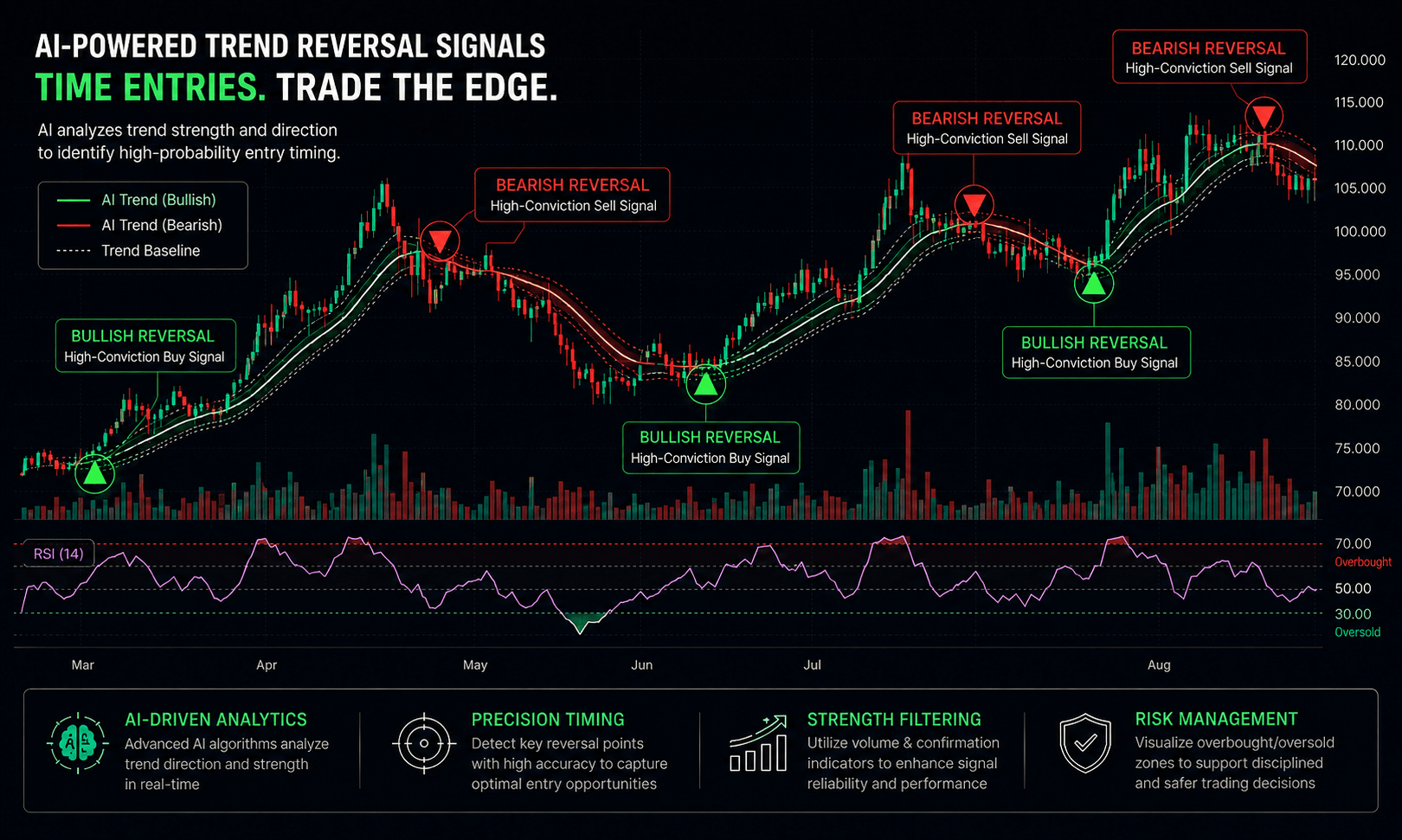
Bull Wave / Bear Wave Forecast Model
Engineered to help you read market direction and momentum faster than the crowd.
- Instantly separate bullish momentum from bearish pressure
- Pinpoint high-probability entry zones with confidence
- Chart signals clear enough for beginners, sharp enough for pros
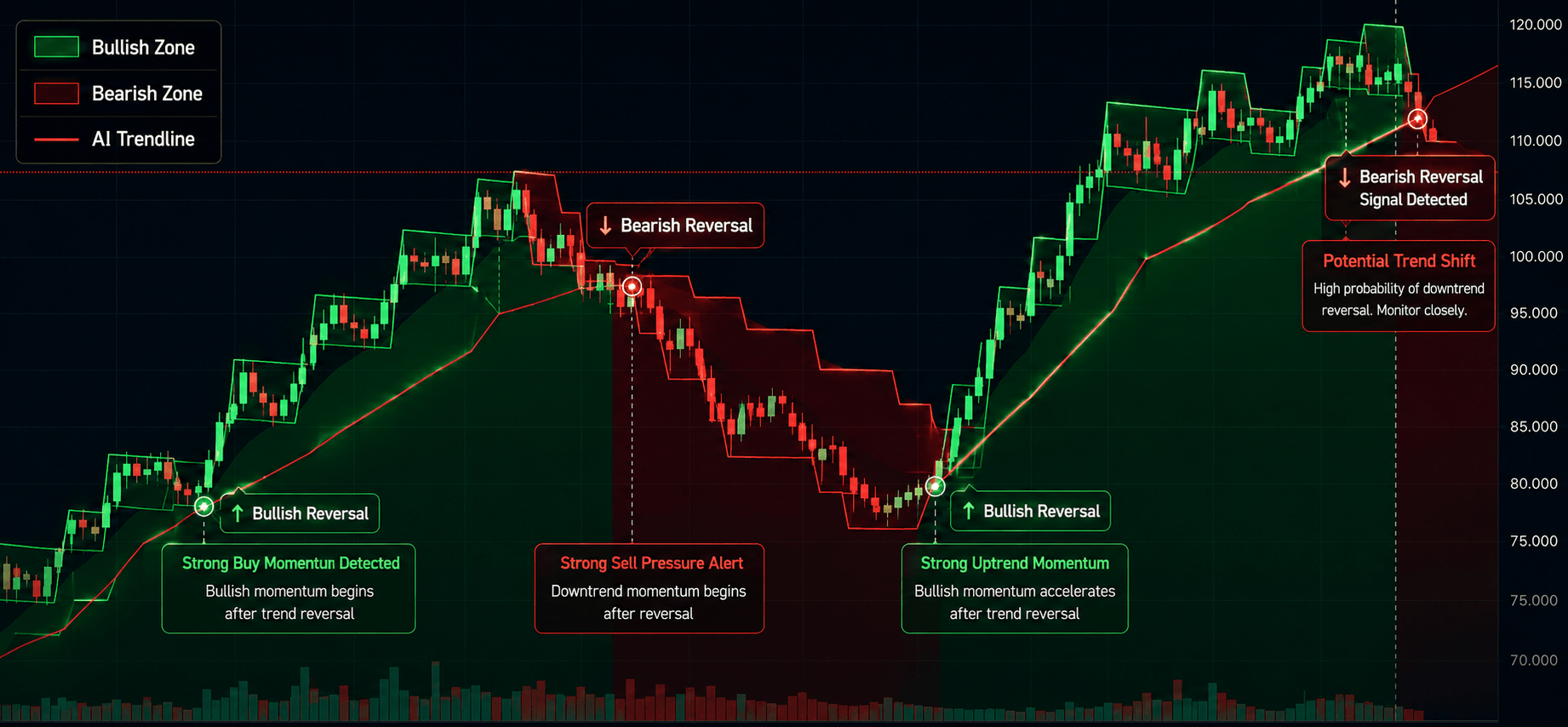
Winning Pattern Detection
Instantly surfaces the high-probability setups that repeat across the charts — a trusted edge for timing your entries and exits.
- Spot momentum building in real time
- Catch trend-reversal points before they break
- Built for active traders who need results, not theory

AI Live Economic Dashboard
AI analyzes real-time market data — turning complex, global investment flows into clear insight in seconds.
- Track global stock markets in real time
- See exactly which assets are strong — and which are fading
- Watch how geopolitical events move the markets
About the Author